Given a frame \({e_{\mu}}\), we can view the dual frame \({\beta^{\mu}}\) as a vector-valued 1-form that simply returns its vector argument: \({\vec{\beta}\left(v\right)\equiv\beta^{\mu}\left(v\right)e_{\mu}=v}\). Clearly this is a frame-independent object. The torsion is then defined to be the exterior covariant derivative

\(\displaystyle \vec{T}\equiv\mathrm{D}\vec{\beta}. \)

In terms of the connection, we must consider \({\vec{\beta}}\) as a frame-dependent \({\mathbb{R}^{n}}\)-valued 1-form, which gives us the torsion as a \({\mathbb{R}^{n}}\)-valued 2-form

\(\displaystyle \vec{T}=\mathrm{d}\vec{\beta}+\check{\Gamma}\wedge\vec{\beta}, \)

This definition of \({\vec{T}}\) is sometimes called Cartan’s first structure equation.

In terms of the covariant derivative, the torsion 2-form is

\begin{aligned}\vec{T}\left(v,w\right) & \equiv\nabla_{v}\left(\vec{\beta}\left(w\right)\right)-\nabla_{w}\left(\vec{\beta}\left(v\right)\right)-\vec{\beta}\left(\left[v,w\right]\right)\\ & =\nabla_{v}w-\nabla_{w}v-\left[v,w\right]. \end{aligned}

For a torsion-free connection in a holonomic frame, we then have \({\nabla_{\sigma}e_{\mu}=\nabla_{\mu}e_{\sigma}}\), which means that the connection coefficients are symmetric in their lower indices, i.e. \({\Gamma^{\lambda}{}_{\mu\sigma}\equiv\beta^{\lambda}\left(\nabla_{\sigma}e_{\mu}\right)=\beta^{\lambda}\left(\nabla_{\mu}e_{\sigma}\right)=\Gamma^{\lambda}{}_{\sigma\mu}}\). For this reason, a torsion-free connection is also called a symmetric connection.

From the definition in terms of the exterior covariant derivative, we can view the torsion as the “sum of the boundary vectors of the surface defined by its arguments after being parallel transported back to \({p}\),” i.e. the torsion measures the amount by which the boundary of a loop fails to close after being parallel transported. From the definition in terms of the covariant derivative, we arrive in the figure below at another interpretation where, like the Lie derivative \({L_{v}w}\), \({\vec{T}(v,w)}\) “completes the parallelogram” formed by its vector arguments, but this parallelogram is formed by parallel transport instead of local flow. Note however that the torsion vector has the opposite sign as the Lie derivative.

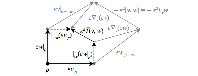
The above depicts how the torsion vector \({\vec{T}\left(v,w\right)}\), constructed starting at the point \({q}\), “completes the parallelogram” formed by parallel transport. \({\Vert_{\varepsilon v}}\) denotes parallel transport along an infinitesimal curve with tangent \({v}\).

Zero torsion then means that moving infinitesimally along \({v}\) followed by the parallel transport of \({w}\) is the same as moving infinitesimally along \({w}\) followed by the parallel transport of \({v}\). Non-zero torsion signifies that “a loop made of parallel transported vectors is not closed.”

As this geometric interpretation suggests, and as is evident from the expression \({\vec{T}\equiv\mathrm{D}\vec{\beta}}\), one can verify algebraically that despite being defined in terms of derivatives \({\vec{T}(v,w)}\) in fact only depends on the local values of \({v}\) and \({w}\), and thus can be viewed as a tensor of type \({\left(1,2\right)}\):

\(\displaystyle T^{c}{}_{ab}v^{a}w^{b}\equiv v^{a}\nabla_{a}w^{c}-w^{a}\nabla_{a}v^{c}-[v,w]^{c} \)

Another relation can be obtained for the torsion tensor by applying its vector value to a function \({f}\) before moving into index notation:

\begin{aligned}\vec{T}\left(v,w\right)(f) & \equiv\left(\nabla_{v}w\right)(f)-\left(\nabla_{w}v\right)(f)-\left[v,w\right](f)\\ \Rightarrow T^{c}{}_{ab}v^{a}w^{b}\nabla_{c}f & =\left(v^{a}\nabla_{a}w^{b}\right)\nabla_{b}f-\left(w^{b}\nabla_{b}v^{a}\right)\nabla_{a}f\\ & \phantom{{}=}-\left[v^{a}\nabla_{a}\left(w^{b}\nabla_{b}f\right)-w^{b}\nabla_{b}\left(v^{a}\nabla_{a}f\right)\right]\\ \Rightarrow T^{c}{}_{ab}\nabla_{c}f & =\nabla_{b}\nabla_{a}f-\nabla_{a}\nabla_{b}f \end{aligned}

Here we have used the Leibniz rule and recalled that \({v(f)=\nabla_{v}f=v^{a}\nabla_{a}f}\) and \({[v,w](f)=v(w(f))-w(v(f))}\). In terms of the connection coefficients \({\Gamma^{c}{}_{ab}=\beta^{c}\nabla_{b}e_{a}}\) we have

\begin{aligned}T^{c}{}_{ab} & =\beta^{c}\vec{T}\left(e_{a},e_{b}\right)\\ & =\beta^{c}\nabla_{a}e_{b}-\beta^{c}\nabla_{b}e_{a}-\beta^{c}[e_{a},e_{b}]\\ & =\Gamma^{c}{}_{ba}-\Gamma^{c}{}_{ab}-[e_{a},e_{b}]^{c}. \end{aligned}

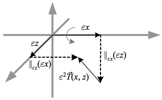
In the above figure, the failure of the parallel transported vectors to meet can be viewed as either due to their lengths changing or due to their being rotated out of the plane of the figure. As we will see, the latter interpretation is more relevant for Riemannian manifolds, where parallel transport leaves lengths invariant. In Einstein-Cartan theory in physics, non-zero torsion is associated with spin in matter. An example along these lines is Euclidean \({\mathbb{R}^{3}}\) with parallel transport defined by translation, except in the \({x}\) direction where parallel transport rotates a vector clockwise by an angle proportional to the distance transported. As we will see in the next section, this parallel transport has torsion but no curvature.

The zero torsion expression \({[v,w]=\nabla_{v}w-\nabla_{w}v}\) means that we can replace partial with covariant derivatives in the usual expression for the Lie derivative of a vector field:

\begin{aligned}\require{cancel}\left(L_{v}w\right)^{a} & =\left[v,w\right]^{a}\\
& =v^{b}\partial_{b}w^{a}-w^{b}\partial_{b}v^{a}\\
& \overset{\cancel{T}}{=}v^{b}\nabla_{b}w^{a}-w^{b}\nabla_{b}v^{a}
\end{aligned}

This can be extended to the Lie derivative of a general tensor, so that in the case of zero torsion we have

\begin{aligned}\require{cancel}L_{v}T^{a_{1}\dots a_{m}}{}_{b_{1}\dots b_{n}} & \overset{\cancel{T}}{=}v^{c}\nabla_{c}T^{a_{1}\dots a_{m}}{}_{b_{1}\dots b_{n}}\\
& \phantom{{}=}-\sum_{j=1}^{m}\left(\nabla_{c}v^{a_{j}}\right)T^{a_{1}\dots a_{j-1}ca_{j+1}\dots a_{m}}{}_{b_{1}\dots b_{n}}\\
& \phantom{{}=}+\sum_{j=1}^{n}\left(\nabla_{b_{j}}v^{c}\right)T^{a_{1}\dots a_{m}}{}_{b_{1}\dots b_{j-1}cb_{j+1}\dots b_{n}}.
\end{aligned}