The Lie derivative \({L_{v}\varphi}\) is defined in terms of a vector field \({v}\), and its value as a “change in \({\varphi}\)” is computed by using \({v}\) to transport the arguments of \({\varphi}\). In contrast, recall that the differential \({\mathrm{d}}\) takes a 0-form \({f\colon M\to\mathbb{R}}\) to a 1-form \({\mathrm{d}f\colon TM\to\mathbb{R}}\) with \({\mathrm{d}f(v)=v(f)}\). Thus \({\mathrm{d}}\) is a derivation of degree +1 on 0-forms, whose value as a “change in \({f}\)” is computed using the vector field argument of the resulting 1-form.
We would like to generalize \({\mathrm{d}}\) to \({k}\)-forms by extending this idea of including the “direction argument” by increasing the degree of the form. It turns out that if we also require the property \({\mathrm{d}\left(\mathrm{d}\left(\varphi\right)\right)=0}\) (or “\({\mathrm{d}^{2}=0}\)”), there is a unique graded derivation of degree +1 that extends \({\mathrm{d}}\) to general \({k}\)-forms; this derivation is called the exterior derivative. We first explore the exterior derivative of a 1-form.
The exterior derivative of a 1-form is defined by
\(\displaystyle \mathrm{d}\varphi\left(v,w\right)\equiv v\left(\varphi\left(w\right)\right)-w\left(\varphi\left(v\right)\right)-\varphi\left(\left[v,w\right]\right),\)
where e.g.
\(\displaystyle v\left(\varphi\left(w\right)\right)=\underset{\varepsilon\rightarrow0}{\textrm{lim}}\frac{1}{\varepsilon}\left[\varphi\left(w\left|_{v_{p}\left(\varepsilon\right)}\right.\right)-\varphi\left(w\left|_{p}\right.\right)\right]\)
measures the change of \({\varphi\left(w\right)}\) in the direction \({v}\), so that
\begin{aligned}\mathrm{d}\varphi\left(v,w\right) & =\underset{\varepsilon\rightarrow0}{\textrm{lim}}\frac{1}{\varepsilon^{2}}\left[\left(\varphi\left(\varepsilon w\left|_{v_{p}\left(\varepsilon\right)}\right.\right)-\varphi\left(\varepsilon w\left|_{p}\right.\right)\right)\right.\\
& \phantom{{=\underset{\varepsilon\rightarrow0}{\textrm{lim}}\frac{1}{\varepsilon^{2}}\left[-\right.}}-\left(\varphi\left(\varepsilon v\left|_{w_{p}\left(\varepsilon\right)}\right.\right)-\varphi\left(\varepsilon v\left|_{p}\right.\right)\right)\\
& \phantom{{=\underset{\varepsilon\rightarrow0}{\textrm{lim}}\frac{1}{\varepsilon^{2}}\left[-\right.}}\left.-\varphi\left(\varepsilon^{2}\left[v,w\right]\right)\right].
\end{aligned}
The term involving the Lie bracket “completes the parallelogram” formed by \({v}\) and \({w}\), so that \({\mathrm{d}\varphi\left(v,w\right)}\) can be viewed as the “sum of \({\varphi}\) on the boundary of the surface defined by its arguments.”
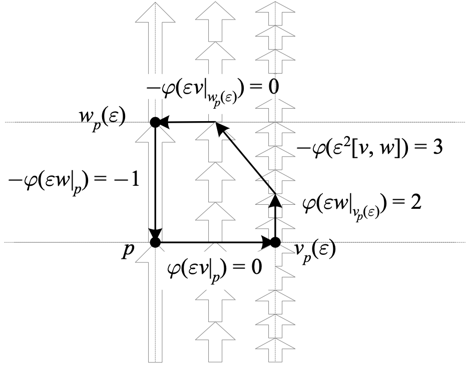
The above depicts the exterior derivative of a 1-form \({\mathrm{d}\varphi\left(v,w\right)}\), which is the sum of \({\varphi}\) along the boundary of the completed parallelogram defined by \({v}\) and \({w}\). So if in the diagram \({\varepsilon=1}\), we have \({\mathrm{d}\varphi\left(v,w\right)=\left(2-1\right)-\left(0-0\right)+3=4}\). This value is valid in the limit \({\varepsilon\rightarrow0}\) if the sum varies like \({\varepsilon^2}\) as depicted in the figure.
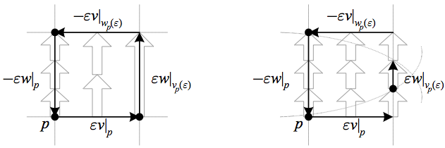
The identity \({\mathrm{d}^{2}=0}\) can then be seen as stating the intuitive fact that the boundary of a boundary is zero. If \({\varphi=\mathrm{d}f}\), then \({\varphi\left(v\right)=\mathrm{d}f\left(v\right)=v\left(f\right)}\), the change in \({f}\) along \({v}\). Thus e.g. \({\varepsilon\varphi\left(v\left|_{p}\right.\right)=f\left(v_{p}\left(\varepsilon\right)\right)-f\left(p\right)}\), so that the value of \({\varphi}\) on \({v}\) is the difference between the values of \({f}\) on the two points which are the boundary of \({v}\). Each endpoint will be cancelled by a starting point as we add up values of \({\varphi}\) along a sequence of vectors, resulting in the difference between the values of \({f}\) at the boundary of the total path defined by these vectors. \({\mathrm{d}\varphi}\) is the value of \({\varphi}\) over the boundary path of the surface defined by its arguments, which has no boundary points and so vanishes.

The above depicts how \({\mathrm{d}^{2}=0}\) corresponds to the boundary of a boundary is zero: each term \({\varphi(v)=\mathrm{d}f(v)}\) is the difference between the values of \({f}\) on the boundary points of \({v}\), which cancel as we traverse the boundary of the surface defined by the arguments of \({\mathrm{d}\varphi(v,w)}\). In the figure we assume a vanishing Lie bracket for simplicity.
Note that \({\mathrm{d}\varphi\left(v,w\right)}\) measures the interaction between \({\varphi}\) and the vector fields \({v}\) and \({w}\), thus avoiding the need to “transport” vectors. In particular, a non-zero exterior derivative can be pictured as resulting from either the vector fields or \({\varphi}\) “changing,” i.e. changing with regard to the implied coordinates of our pictures.
The above depicts a non-zero exterior derivative \({\mathrm{d}\varphi\left(v,w\right)}\), which results from changes in \({\varphi\left(v\right)}\) or \({\varphi\left(w\right)}\), not changes in either \({\varphi}\) or the vector fields alone as compared to some transport.
If we calculate \({\mathrm{d}\varphi\left(e_{1},e_{2}\right)}\) explicitly in a holonomic frame in two dimensions, \({\mathrm{d}\left(\varphi_{1}\mathrm{d}x^{1}+\varphi_{2}\mathrm{d}x^{2}\right)=\mathrm{d}\varphi_{1}\wedge \mathrm{d}x^{1}+\mathrm{d}\varphi_{2}\wedge \mathrm{d}x^{2}}\), so applying this to the basis vector fields \({e_{1}}\) and \({e_{2}}\) we have
\begin{aligned}\mathrm{d}\varphi\left(e_{1},e_{2}\right) & =\mathrm{d}\varphi_{1}\left(e_{1}\right)\cdot \mathrm{d}x^{1}\left(e_{2}\right)-\mathrm{d}\varphi_{1}\left(e_{2}\right)\cdot \mathrm{d}x^{1}\left(e_{1}\right)\\
& \phantom{{}=}+\mathrm{d}\varphi_{2}\left(e_{1}\right)\cdot \mathrm{d}x^{2}\left(e_{2}\right)-\mathrm{d}\varphi_{2}\left(e_{2}\right)\cdot \mathrm{d}x^{2}\left(e_{1}\right)\\
& =e_{1}\left(\varphi_{2}\right)-e_{2}\left(\varphi_{1}\right)\\
& =\frac{\partial\varphi_{2}}{\partial x^{1}}-\frac{\partial\varphi_{1}}{\partial x^{2}}.
\end{aligned}
Note that a holonomic dual frame \({\beta^{\mu}=\mathrm{d}x^{\mu}}\) satisfies \({\mathrm{d}\beta^{\mu}=\mathrm{dd}x^{\mu}=0}\). In an anholonomic frame, we have
\begin{aligned}\mathrm{d}\varphi\left(e_{1},e_{2}\right)&=e_{1}\left(\varphi\left(e_{2}\right)\right)-e_{2}\left(\varphi\left(e_{1}\right)\right)-\varphi\left(\left[e_{1},e_{2}\right]\right)\\&=\mathrm{d}\varphi_{2}\left(e_{1}\right)-\mathrm{d}\varphi_{1}\left(e_{2}\right)-\varphi_{1}\left[e_{1},e_{2}\right]^{1}-\varphi_{2}\left[e_{1},e_{2}\right]^{2}\\\Rightarrow\mathrm{d}\beta^{\mu}\left(e_{1},e_{2}\right)&=-\left[e_{1},e_{2}\right]^{\mu}\\\Rightarrow\mathrm{d}\beta^{\mu}&=-\frac{1}{2}\left[e_{\nu},e_{\lambda}\right]^{\mu}\beta^{\nu}\land\beta^{\lambda}.\end{aligned}