Geometrically, the Ricci function \({\mathrm{Ric}(v)}\) at a point \({p\in M^{n}}\) can be seen to measure the extent to which the area defined by the geodesics emanating from the \({(n-1)}\)-surface perpendicular to \({v}\) changes in the direction of \({v}\). Considering the three dimensional case in an orthonormal frame (and again dropping the hats in \({\hat{e}_{i}}\) to avoid clutter), we have
\(\displaystyle \begin{aligned}\mathrm{Ric}(e_{2}) & =\left\langle \check{R}(e_{1},e_{2})\vec{e}_{2},e_{1}\right\rangle +\left\langle \check{R}(e_{3},e_{2})\vec{e}_{2},e_{3}\right\rangle \\ & =K(e_{1},e_{2})+K(e_{3},e_{2}). \end{aligned} \)
If we form a cube made from parallel transported vectors as we did for the first Bianchi identity, we can see that each sectional curvature term in \({\mathrm{Ric}(e_{2})}\) takes an edge of the cube and measures the length of the difference between the cube-aligned component of its parallel transport in the \({e_{2}}\) direction and the edge of the cube at a point parallel transported in the \({e_{2}}\) direction.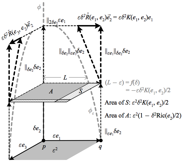
The above depicts how each sectional curvature measures the convergence of geodesics, while their sum forms the Ricci curvature function, which measures the change in the area of the \({(n-1)}\)-surface formed by geodesics perpendicular to its argument. In the figure we assume without loss of generality (see below) that \({\check{R}(e_{1},e_{2})\vec{e}_{2}}\) is parallel to \({e_{1}}\).
The figure above details the sectional curvature \({K(e_{1},e_{2})=\beta^{1}\check{R}(e_{1},e_{2})\vec{e}_{2}}\) assuming that \({\check{R}(e_{1},e_{2})\vec{e}_{2}}\) is parallel to \({e_{1}}\), so that \({\left\langle \check{R}(e_{1},e_{2})\vec{e}_{2},e_{1}\right\rangle =\left\Vert \check{R}(e_{1},e_{2})\vec{e}_{2}\right\Vert }\). The parallel transport of \({e_{2}}\) along itself is depicted as parallel, so that the geodesic parametrized by arclength \({\phi(t)}\) is a straight line in the figure. The vector \({\parallel_{\delta e_{2}}\parallel_{\varepsilon e_{1}}\delta e_{2}}\) is the parallel transport of \({\parallel_{\varepsilon e_{1}}\delta e_{2}}\) by \({\delta}\) in the direction parallel to \({e_{2}}\), and therefore the geodesic \({\phi_{\varepsilon}(t)}\) tangent to \({\parallel_{\varepsilon e_{1}}\delta e_{2}}\) at \({q}\) has tangent \({\parallel_{\delta e_{2}}\parallel_{\varepsilon e_{1}}\delta e_{2}}\) after moving a distance \({\delta}\). If we consider the function \({f(t)}\) whose value at \({t=\delta}\) is the quantity \({(L-\varepsilon)}\) in the figure (i.e. \({f(t)}\) measures the offset of the geodesic from the right edge of the stack of parallel cubes), its derivative is the slope of the tangent, so that to lowest order in \({t}\) we have
\(\displaystyle \begin{aligned}\dot{f}(t) & =-\varepsilon t^{2}K(e_{1},e_{2})/t\\ & =-\varepsilon tK(e_{1},e_{2})\\ \Rightarrow f(t) & =-\varepsilon t^{2}K(e_{1},e_{2})/2. \end{aligned} \)
We can generalize this logic to arbitrary unit vectors \({\hat{v}}\) and \({\hat{w}}\) to conclude that \({K(\hat{v},\hat{w})/2}\) is the “fraction by which the geodesic parallel to \({\hat{w}}\) with separation direction \({\hat{v}}\) bends towards \({\hat{w}}\).” More precisely, in terms of the distance function and the exponential map, to order \({\varepsilon}\) and \({\delta^{2}}\) we have
\(\displaystyle d\left(\mathrm{exp}(\delta\hat{w}),\mathrm{exp}(\delta\parallel_{\varepsilon\hat{v}}\hat{w})\right)=\varepsilon\left(1-\frac{\delta^{2}}{2}K(\hat{v},\hat{w})\right). \)
In the general case \({L}\) in the figure is the distance between two geodesics infinitesimally separated in the \({\hat{v}}\) direction, so if we define \({L(t)}\) as this distance at any point along the parametrized geodesic tangent to \({\hat{w}}\), the above becomes
\(\displaystyle \begin{aligned}L(t) & =L(0)\left(1-\frac{t^{2}}{2}K(\hat{v},\hat{w})\right)\\ \Rightarrow\left.\frac{\ddot{L}}{L}\right|_{t=0} & =-K(\hat{v},\hat{w}), \end{aligned} \)
where the double dots indicate the second derivative with respect to \({t}\). Thus \({K(\hat{v},\hat{w})}\) is “the acceleration of two parallel geodesics in the \({\hat{w}}\) direction with initial separation direction \({\hat{v}}\) towards each other as a fraction of the initial gap.”
Now, the distance \({\left|\varepsilon-L\right|=\varepsilon\delta^{2}K(e_{1},e_{2})/2}\) defines a strip \({S}\) bordering the surface orthogonal to \({e_{2}}\) a distance \({\delta}\) in the \({e_{2}}\) direction. This strip thus has an area \({\varepsilon^{2}\delta^{2}K(e_{1},e_{2})/2}\). If we sum this with the other strip of area \({\varepsilon^{2}\delta^{2}K(e_{3},e_{2})/2}\), to order \({\varepsilon^{2}}\) and \({\delta^{2}}\) we measure the extent to which the area \({A}\) defined by the geodesics emanating from the surface perpendicular to \({e_{2}}\) changes in the direction of \({e_{2}}\). But the sum of sectional curvatures is just the Ricci function, so that in general \({\mathrm{Ric}(v)/2}\) is the “fraction by which the area defined by the geodesics emanating from the \({(n-1)}\)-surface perpendicular to \({v}\) changes in the direction of \({v}\).” More precisely, we can follow the same logic as above, defining the “infinitesimal geodesic \({(n-1)}\)-area” \({A(t)}\) along a parametrized geodesic tangent to \({v}\), so that to order \({\varepsilon^{2}}\) and \({t^{2}}\) we have
\(\displaystyle \begin{aligned}A(t) & =\varepsilon^{2}\left(1-\frac{t^{2}}{2}\mathrm{Ric}(v)\right)\\ \Rightarrow\left.\frac{\ddot{A}}{A}\right|_{t=0} & =-\mathrm{Ric}(v). \end{aligned} \)
Thus \({\mathrm{Ric}(v)}\) is “the acceleration of the parallel geodesics emanating from the \({(n-1)}\)-surface perpendicular to \({v}\) towards each other as a fraction of the initial surface.” Note that if our previous assumption that \({\check{R}(e_{1},e_{2})\vec{e}_{2}}\) is parallel to \({e_{1}}\) is dropped, the only impact is that of an \({e_{3}}\) component on the area calculation; to address this, a more accurate picture would be to extend the area to include all four quadrants defined by both negative and positive values of \({e_{1}}\) and \({e_{3}}\), in which case any change in area due to an \({e_{3}}\) component cancels. In the case of a pseudo-Riemannian manifold, “areas” and “volumes” become less geometric concepts; however, we have a clear picture in the case of a Lorentzian manifold that the Ricci function applied to a time-like vector \({v\equiv\partial/\partial x^{0}=\partial/\partial t}\) tells us how the infinitesimal space-like volume \({V}\) of free-falling particles (i.e. following geodesics) changes over time according to \({\ddot{V}/V=-\mathrm{Ric}(v)=-R_{00}=-R^{\mu}{}_{0\mu0}}\).