Now let us consider a vector field \({J(t)}\) along the geodesic \({\phi(t)}\) such that \({J(0)\equiv J\left|_{p}\right.=J\left|_{\phi(0)}\right.=e_{1}}\) and \({J(\delta)\equiv J\left|_{\phi(\delta)}\right.=(L/\varepsilon)\parallel_{\delta e_{2}}e_{1}}\), i.e. \({J}\) is the vector field “between adjacent geodesics.”
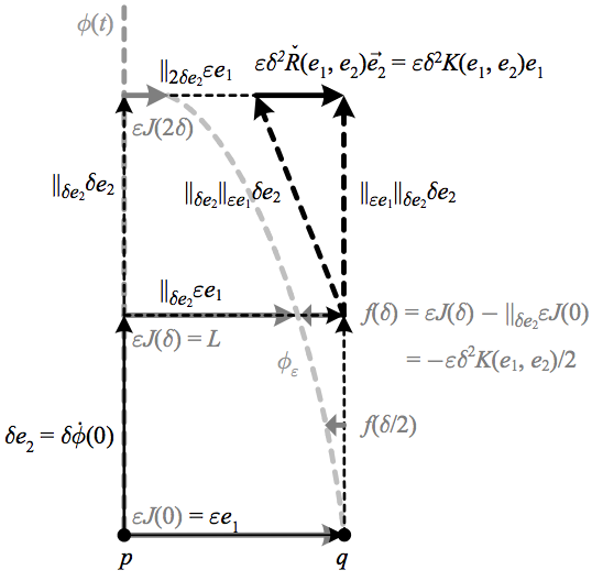
The above depicts how a Jacobi field is the vector field between adjacent geodesics, whose construction creates a relationship between the covariant derivative and the sectional curvature.
Then the function \({f(t)=-\varepsilon t^{2}K(e_{1},e_{2})/2=-\varepsilon t^{2}K(J,\dot{\phi})/2}\) is the difference between \({J}\) and its parallel transport in the direction tangent to \({\phi}\), i.e. it is the value of the covariant derivative along \({\phi}\). Since this difference is of order \({t^{2}}\), at \({t=0}\) we have \({\mathrm{D}_{t}^{2}J=-K(J,\dot{\phi})}\), or dropping the assumption that \({\check{R}(e_{1},e_{2})\vec{e}_{2}}\) is parallel to \({e_{1}}\),
\(\displaystyle \frac{\mathrm{D}^{2}J}{\mathrm{d}t^{2}}+\check{R}(J,\dot{\phi})\vec{\dot{\phi}}=0. \)
Considered as an equation for all \({J(t)}\), this is called the Jacobi equation, with the vector field \({J(t)}\) that satisfies it called a Jacobi field. A more precise way to generalize our construction of \({J}\) is to define a one-parameter family of geodesics \({\phi_{s}(t)}\), so that
\(\displaystyle J(t)=\left.\frac{\partial\phi_{s}(t)}{\partial s}\right|_{s=0}. \)
If \({M}\) is complete then every Jacobi field can be expressed in this way for some family of geodesics.
If we then consider the Jacobi fields \({J_{v}(t)}\) corresponding to the geodesics \({\phi_{v}(t)}\) of tangent vectors \({\left\Vert v\right\Vert =1}\) parametrized by arclength and such that to order \({t}\) we have \({\left\Vert J_{v}(1)\right\Vert =1}\), it can be shown ([3] pp. 114-115) that to order \({t^{3}}\) we have \({\left\Vert J_{v}(t)\right\Vert =t(1-t^{2}K(J_{v},\dot{\phi}_{v})/6)}\).
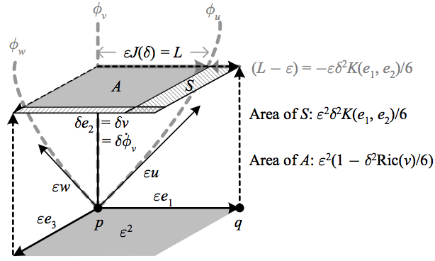
The above depicts how the infinitesimal geodesic area element can be derived from the Jacobi field between radial geodesics.
This means that if we apply the previous reasoning for parallel geodesics to these radial geodesics we have an “infinitesimal geodesic \({(n-1)}\)-area element” \({A(t)=t^{2}(1-t^{2}\mathrm{Ric}(v)/6)}\). Integrating this over all values of \({v}\) gives for small \({t=\varepsilon}\) the surface area of a geodesic \({n}\)-ball of radius \({\varepsilon}\), which we denote \({\partial B_{\varepsilon}(M^{n})}\). But this integral just averages the values of the Ricci function, which is the Ricci scalar over the dimension \({n}\), so that to order \({\varepsilon^{2}}\) we have
\(\displaystyle \frac{\partial B_{\varepsilon}(M^{n})}{\partial B_{\varepsilon}(\mathbb{R}^{n})}=1-\frac{\varepsilon^{2}}{6n}R, \)
and integrating over the radius we find (see [10]) a similar relation for the volume of a geodesic sphere compared to a Euclidean one of
\(\displaystyle \frac{B_{\varepsilon}(M^{n})}{B_{\varepsilon}(\mathbb{R}^{n})}=1-\frac{\varepsilon^{2}}{6(n+2)}R. \)
Thus \({\varepsilon^{2}R/6n}\) is “the fraction by which the surface area of a geodesic \({n}\)-ball of radius \({\varepsilon}\) is smaller than it would be under a flat metric,” and \({\varepsilon^{2}R/6(n+2)}\) is “the fraction by which the volume of a geodesic \({n}\)-ball of radius \({\varepsilon}\) is smaller than it would be under a flat metric.”
Alternatively, we can use Riemann normal coordinates to express \({v}\) in our “infinitesimal geodesic \({(n-1)}\)-area element,” whereupon following similar logic to the above we find that, at points close to the origin of our coordinates, to order \({\left\Vert x\right\Vert ^{2}}\) the volume element is
\(\displaystyle \mathrm{d}V=\left(1-\frac{1}{6}R_{\mu\nu}x^{\mu}x^{\nu}\right)\mathrm{d}x^{1}\cdots\mathrm{d}x^{n}, \)
or using the expression of the volume element in terms the square root of the determinant of the metric, again to order \({\left\Vert x\right\Vert ^{2}}\) we find that
\(\displaystyle g_{\mu\nu}=\delta_{\mu\nu}-\frac{1}{3}R_{\mu\lambda\nu\sigma}x^{\lambda}x^{\sigma}. \)
As is apparent from their definitions, the Ricci tensor and function do not depend on the metric. We can attempt to find a metric-free geometric interpretation by considering the concept of a parallel volume form. This is defined as a volume form which is invariant under parallel transport. We immediately see that it is only possible to define such a form if parallel transport around a loop does not alter volumes, i.e. that \({\check{R}}\) must be \({o(r,s)}\)-valued. This means that the connection is metric compatible, so we can define one if we wish; but if we do not, and assume zero torsion so that the Ricci tensor is symmetric, then our logic for volumes remains valid and we can still take a metric-free view of the expression for \({\mathrm{d}V}\) above as expressing the geodesic volume as measured by the parallel volume form. Note that unlike the Ricci tensor and function, the definitions here of the individual sectional curvatures and scalar curvature do depend upon the metric.