Recall that the divergence of a vector field \({u}\) can be generalized to a pseudo-Riemannian manifold of signature \({\left(r,s\right)}\) by defining \({\mathrm{div}(u)\equiv(-1)^{s}*\mathrm{d}(*(u^{\flat}))}\). Also recalling that \({i_{u}\Omega=*(u^{\flat})}\) and \({(-1)^{s}A=(*A)\Omega}\) for \({A\in\Lambda^{n}M^{n}}\), we have \({\mathrm{d}(i_{u}\Omega)=\mathrm{d}(*(u^{\flat}))=(-1)^{s}*\mathrm{d}(*(u^{\flat}))\Omega=\mathrm{div}(u)\Omega}\). Using \({i_{u}\mathrm{d}+\mathrm{d}i_{u}=L_{u}}\) we then arrive at \({\mathrm{div}(u)\Omega=L_{u}\Omega}\), or as it is more commonly written

\(\displaystyle \mathrm{div}(u)\mathrm{d}V=L_{u}\mathrm{d}V. \)

Thus we can say that \({\mathrm{div}(u)}\) is “the fraction by which a unit volume changes when transported by the flow of \({u}\),” and if \({\mathrm{div}(u)=0}\) then we can say that “the flow of \({u}\) leaves volumes unchanged.” Expanding the volume element in coordinates \({x^{\lambda}}\) we can obtain an expression for the divergence in terms of these coordinates,

\(\displaystyle \mathrm{div}(u)=\frac{1}{\sqrt{\left|\mathrm{det}(g)\right|}}\partial_{\lambda}\left(\sqrt{\left|\mathrm{det}(g)\right|}u^{\lambda}\right). \)

Note that both this metric-dependent expression and the expression \({\nabla_{a}u^{a}}\) (sometimes called the covariant divergence) in terms of the Levi-Civita connection are coordinate-independent and equal to \({\partial_{a}u^{a}}\) in Riemann normal coordinates, confirming our expectation that for zero torsion we have

\(\require{cancel}\displaystyle \mathrm{div}(u)=\overline{\nabla}_{a}u^{a}. \)

Recall however that the connection coefficients do not vanish in Riemann normal coordinates for non-zero torsion; in this case we can use the contorsion tensor contraction \({K^{a}{}_{ba}=T^{a}{}_{ab}}\) to relate the pseudo-Riemannian divergence to the covariant divergence by

\(\displaystyle \mathrm{div}(u) =\nabla_{a}u^{a}-T^{a}{}_{ab}u^{b}. \)

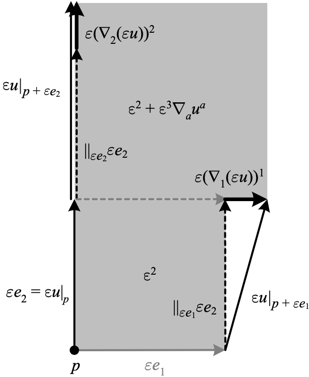
The divergence measures the change in volume due to the flow. Here we assume the vector field \({u}\) has unit length at point \({p}\), and choose an orthonormal frame which aligns \({e_{2}}\) with \({u}\). Each covariant derivative extends a face of the volume, with their sum being proportional to the total change in volume. Note that the upper right corner is of order \({\varepsilon^{4}}\) and so can be neglected, and e.g. any component of \({\nabla_{1}u}\) orthogonal to \({e_{1}}\) leaves the volume unchanged, since a more accurate depiction would include the volume with edge \({-\varepsilon e_{1}}\), where by linearity this component would be in the opposite direction and thus cancel the volume change. Also note that non-zero torsion would reduce the top edge \({\parallel_{\varepsilon e_{2}}\varepsilon e_{1}}\) by \({\varepsilon^{2}T^{1}{}_{1b}u^{b}}\), which must be added back by subtracting this component, matching the algebraic result.

Using the relation \({\mathrm{div}(u)\Omega=\mathrm{d}(i_{u}\Omega)}\) above, along with Stokes’ theorem, we again recover the classical divergence theorem

\(\displaystyle \begin{aligned}\int_{V}\mathrm{div}(u)\mathrm{d}V & =\int_{\partial V}i_{u}\mathrm{d}V\\ & =\int_{\partial V}\left\langle u,\hat{n}\right\rangle \mathrm{d}S, \end{aligned} \)

where \({V}\) is an \({n}\)-dimensional compact submanifold of \({M^{n}}\), \({\hat{n}}\) is the unit normal vector to \({\partial V}\), and \({\mathrm{d}S\equiv i_{\hat{n}}\mathrm{d}V}\) is the induced volume element (“surface element”) for \({\partial V}\). In the case of a Riemannian metric, this can be thought of as reflecting the intuitive fact that “the change in a volume due to the flow of \({u}\) is equal to the net flow across that volume’s boundary.” If \({\mathrm{div}(u)=0}\) then we can say that “the net flow of \({u}\) across the boundary of a volume is zero.” We can also consider an infinitesimal \({V}\), so that the divergence at a point measures “the net flow of \({u}\) across the boundary of an infinitesimal volume.”

In physics, one considers the divergence of the current vector (AKA current density, flux, flux density) \({j\equiv\rho u}\) of a physical flow in space at a moment in time, where \({\rho}\) is the density of the physical quantity \({Q}\) and \({u}\) is thus a velocity field; e.g. in \({\mathbb{R}^{3}}\), \({j}\) has units \({Q/(\mathrm{length})^{2}(\mathrm{time})}\). For a flat Riemannian metric on the manifold representing space, the continuity equation (AKA equation of continuity) is

\(\displaystyle \frac{\mathrm{d}q}{\mathrm{d}t}=\Sigma-\int_{\partial V}\left\langle j,\hat{n}\right\rangle \mathrm{d}S, \)

where \({q}\) is the amount of \({Q}\) contained in \({V}\), \({t}\) is time, and \({\Sigma}\) is the rate of \({Q}\) being created within \({V}\). The continuity equation thus states the intuitive fact that the change of \({Q}\) within \({V}\) equals the amount generated less the amount which passes through \({\partial V}\).

Using the divergence theorem, we can then obtain the differential form of the continuity equation

\(\displaystyle \frac{\partial\rho}{\partial t}=\sigma-\mathrm{div}(j), \)

where \({\sigma}\) is the amount of \({Q}\) generated per unit volume per unit time. This equation then states the intuitive fact that at a point, the change in density of \({Q}\) equals the amount generated less the amount that moves away. Positive \({\sigma}\) is referred to as a source of \({Q}\), and negative \({\sigma}\) a sink. If \({\sigma=0}\) then we say that \({Q}\) is a conserved quantity and refer to the continuity equation as a (local) conservation law.

Under a flat Lorentzian metric, we can combine \({\rho}\) and \({j}\) into the four-current

\(\displaystyle J\equiv(\rho,j^{\mu}), \)

and express the continuity equation with \({\sigma=0}\) as

\(\displaystyle \mathrm{div}(J)=0, \)

whereupon \({J}\) is called a conserved current. Note that if any curvature is present, when we split out the time component we recover a Riemannian divergence but introduce a source due to the non-zero Christoffel symbols

\(\displaystyle \begin{aligned}\overline{\nabla}_{\mu}J^{\mu}&=\partial_{\mu}J^{\mu}+\overline{\Gamma}^{\mu}{}_{\nu\mu}J^{\nu}\\&=\partial_{t}\rho+\overline{\nabla}_{i}j^{i}+\left(\overline{\Gamma}^{\mu}{}_{t\mu}\rho+\overline{\Gamma}^{t}{}_{it}j^{i}\right),\end{aligned} \)

where \({t}\) is the negative signature component and the index \({i}\) goes over the remaining positive signature components. Thus, since the Christoffel symbols are coordinate-dependent, in the presence of curvature there is in general no coordinate-independent conserved quantity associated with a vanishing Lorentzian divergence. A conserved current nevertheless means that the quantity is conserved in finite volumes of spacetime, in the sense that \({\int_{\partial V}\left\langle J,\hat{n}\right\rangle \mathrm{d}S=0}\) over any spacetime volume \({V}\), and the continuity equation holds for the components of the coordinate-dependent quantity \({\mathfrak{J}\equiv J\sqrt{\left|\mathrm{det}(g)\right|}}\), since

\begin{aligned}\partial_{\mu}\mathfrak{J}^{\mu} & =\partial_{t}\mathfrak{J}^{t}+\partial_{i}\mathfrak{J}^{i}\\
& =\partial_{t}\mathfrak{J}^{t}+\overline{\nabla}_{i}\mathfrak{J}^{i}=0.
\end{aligned}

More details on the divergence, currents, and conservation laws may be found in an Appendix.