The exterior covariant derivative \({\mathrm{D}}\) parallel transports its values on the boundary before summing them, and therefore we do not expect it to mimic the property \({\mathrm{d}^{2}=0}\). Indeed it does not; instead, for a vector field \({w}\) viewed as a vector-valued 0-form \({\vec{w}}\), we have

\(\displaystyle \left(\mathrm{D}^{2}\vec{w}\right)(u,v)\equiv\check{R}\left(u,v\right)\vec{w}=\nabla_{u}\nabla_{v}w-\nabla_{v}\nabla_{u}w-\nabla_{\left[u,v\right]}w, \)

which defines the curvature 2-form \({\check{R}}\), which is \({gl(\mathbb{R}^{n})}\)-valued. From its definition, \({\check{R}\vec{w}}\) is a frame-independent quantity, and thus if \({\vec{w}}\) is considered as a vector-valued 0-form, \({\check{R}}\) is frame-independent as well. In the (more common) case that we view \({\vec{w}}\) as a frame-dependent \({\mathbb{R}^{n}}\)-valued 0-form, \({\check{R}}\) must be considered to be \({gl(n,\mathbb{R})}\)-valued, and is thus a frame-dependent matrix, transforming under a (frame-dependent) \({GL(n,\mathbb{R})}\)-valued 0-form \({\check{\gamma}^{-1}}\) change of frame like

\(\displaystyle \left(\check{R}\right)^{\prime}=\check{\gamma}\check{R}\check{\gamma}^{-1}. \)

A connection with zero curvature is called flat, as is any region of \({M}\) with a flat connection.

For a general \({\mathbb{R}^{n}}\)-valued form \({\vec{\varphi}}\) it is not hard to arrive at an expression for \({\check{R}}\) in terms of the connection:

\(\displaystyle \mathrm{D}^{2}\vec{\varphi}=\left(\mathrm{d}\check{\Gamma}+\check{\Gamma}\wedge\check{\Gamma}\right)\wedge\vec{\varphi}=\check{R}\wedge\vec{\varphi} \)

Note that \({\mathrm{D}\check{\Gamma}=\mathrm{d}\check{\Gamma}+\check{\Gamma}[\wedge]\check{\Gamma}}\) is a similar but distinct construction, since \({(\check{\Gamma}\wedge\check{\Gamma})\left(v,w\right)=\check{\Gamma}\left(v\right)\check{\Gamma}\left(w\right)-\check{\Gamma}\left(w\right)\check{\Gamma}\left(v\right)}\), while \({(\check{\Gamma}[\wedge]\check{\Gamma})\left(v,w\right)=[\check{\Gamma}\left(v\right),\check{\Gamma}\left(w\right)]-[\check{\Gamma}\left(w\right),\check{\Gamma}\left(v\right)]=2(\check{\Gamma}\wedge\check{\Gamma})\left(v,w\right)}\). Thus we can equivalently define

\begin{aligned}\check{R} & \equiv\mathrm{d}\check{\Gamma}+\check{\Gamma}\wedge\check{\Gamma}\\ & =\mathrm{d}\check{\Gamma}+\frac{1}{2}\check{\Gamma}[\wedge]\check{\Gamma}. \end{aligned}

The definition of \({\check{R}}\) in terms of \({\check{\Gamma}}\) is sometimes called Cartan’s second structure equation. An immediate property from the definition of \({\check{R}}\) is \({\check{R}(u,v)=-\check{R}(v,u)}\), which allows us to write e.g. for a vector-valued 1-form \({\vec{\varphi}}\)

\begin{aligned}\left(\mathrm{D}^{2}\vec{\varphi}\right)(u,v,w) & =\left(\check{R}\wedge\vec{\varphi}\right)\left(u,v,w\right)\\ & =\check{R}\left(u,v\right)\vec{\varphi}(w)+\check{R}\left(v,w\right)\vec{\varphi}(u)+\check{R}\left(w,u\right)\vec{\varphi}(v). \end{aligned}

Constructing the same picture as we did for the double exterior derivative, we put \({\mathrm{D}^{2}\vec{w}\equiv\mathrm{D}\vec{\varphi}}\), where \({\vec{\varphi}(v)\equiv\mathrm{D}\vec{w}(v)=\nabla_{v}w}\). Expanding both derivatives in terms of parallel transport, we find in the following figure that as we sum values around the boundary of the surface defined by its arguments, \({\mathrm{D}^{2}}\) fails to cancel the endpoint and starting point at the far corner. Examining the values of these non-canceling points, we can view the curvature as “the difference between \({w}\) when parallel transported around the two opposite edges of the boundary of the surface defined by its arguments.”

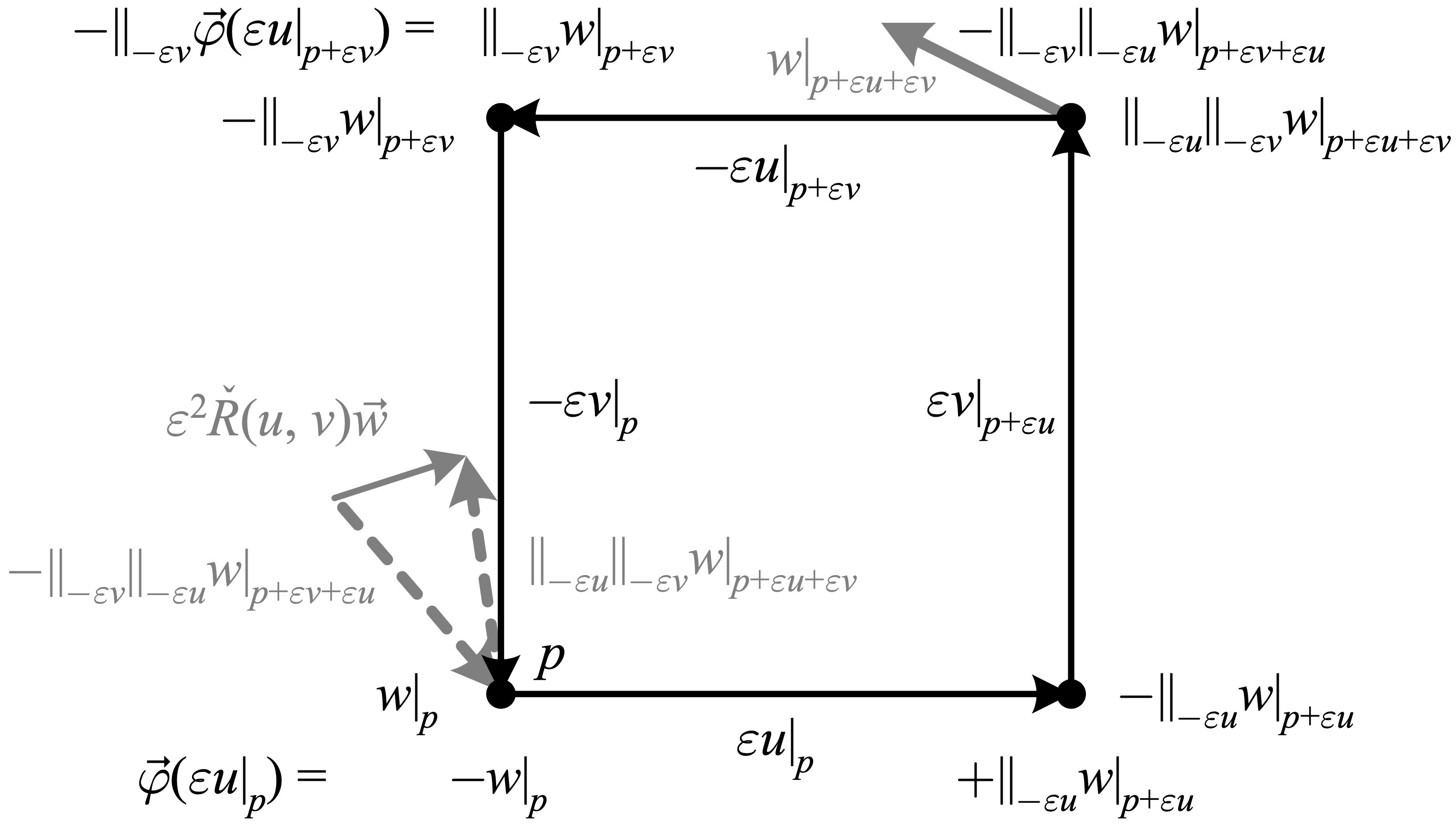
The above depicts how \({\check{R}\left(u,v\right)\vec{w}=\left(\mathrm{D}^{2}\vec{w}\right)(u,v)}\) is “the difference between \({w}\) when parallel transported around the two opposite edges of the boundary of the surface defined by its arguments.” In the figure we assume vanishing Lie bracket for simplicity, so that \({v\left|_{p+\varepsilon u+\varepsilon v}\right.=v\left|_{p+\varepsilon v+\varepsilon u}\right.}\).

In terms of the connection, we can use the path-ordered exponential formulation to examine the parallel transporter around the closed path \({L\equiv\partial S}\) defined by the surface \({S\equiv\left(\varepsilon u\wedge\varepsilon v\right)}\) to order \({\varepsilon^{2}}\). This calculation after some work (see [9] pp. 51-53) yields

\(\displaystyle \parallel_{L}(w)=P\textrm{exp}\left(-\int_{L}\check{\Gamma}\right)\vec{w}=w-\int_{S}\left(\mathrm{d}\check{\Gamma}+\check{\Gamma}\wedge\check{\Gamma}\right)\vec{w}=w-\varepsilon^{2}\check{R}\left(u,v\right)\vec{w}, \)

where we have dropped the indices since \({L}\) is a closed path and thus \({\parallel_{L}}\) is basis-independent. Thus the curvature can be viewed as “the difference between \({w}\) and its parallel transport around the boundary of the surface defined by its arguments.”

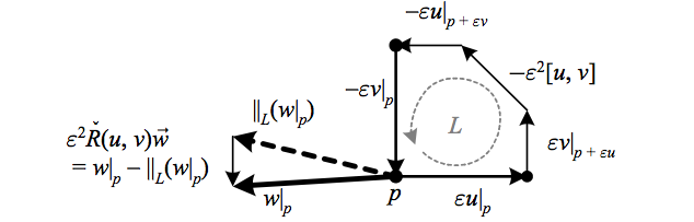
The above depicts how \({\check{R}\left(u,v\right)\vec{w}}\) is “the difference between \({w}\) and its parallel transport around the boundary of the surface defined by its arguments.”

As these pictures suggest, one can verify algebraically that the value of \({\check{R}\left(u,v\right)\vec{w}}\) at a point \({p}\) only depends upon the value of \({w}\) at \({p}\), even though it can be defined in terms of \({\nabla w}\), which depends upon nearby values of \({w}\). Similarly, \({\check{R}\left(u,v\right)\vec{w}}\) at a point \({p}\) only depends upon the values of \({u}\) and \({v}\) at \({p}\), even though it can be defined in terms of \({[u,v]}\), which depends upon their vector field values (note that \({\nabla_{u}\nabla_{v}w}\) depends upon the vector field values of both \({v}\) and \({w}\)). Finally, \({\check{R}}\) (as a \({gl(\mathbb{R}^{n})}\)-valued 2-form) is frame-independent, even though it can be defined in terms of \({\check{\Gamma}}\), which is not. Thus the curvature can be viewed as a tensor of type \({\left(1,3\right)}\), called the Riemann curvature tensor (AKA Riemann tensor, curvature tensor, Riemann–Christoffel tensor):

\begin{aligned}R^{c}{}_{dab}u^{a}v^{b}w^{d} & = u^{a}\nabla_{a}\left(v^{b}\nabla_{b}w^{c}\right)-v^{b}\nabla_{b}\left(u^{a}\nabla_{a}w^{c}\right)-[u,v]^{d}\nabla_{d}w^{c}\\ & =u^{a}v^{b}\nabla_{a}\nabla_{b}w^{c}-u^{a}v^{b}\nabla_{b}\nabla_{a}w^{c}+T^{d}{}_{ab}u^{a}v^{b}\nabla_{d}w^{c}\\ \Rightarrow R^{c}{}_{dab}w^{d} & =\left(\nabla_{a}\nabla_{b}-\nabla_{b}\nabla_{a}+T^{d}{}_{ab}\nabla_{d}\right)w^{c} \end{aligned}

Here we have used the Leibniz rule and recalled that \({[u,v]^{d}=u^{a}\nabla_{a}v^{d}-v^{b}\nabla_{b}u^{d}-T^{d}{}_{ab}u^{a}v^{b}}\). To obtain an expression in terms of the connection coefficients, we first examine the double covariant derivative, recalling that \({\nabla_{b}w^{c}}\) is a tensor:

\begin{aligned}\nabla_{a}\left(\nabla_{b}w^{c}\right) & =\partial_{a}\nabla_{b}w^{c}+\Gamma^{c}{}_{fa}\nabla_{b}w^{f}-\Gamma^{f}{}_{ba}\nabla_{f}w^{c}\\ & =\partial_{a}\partial_{b}w^{c}+\partial_{a}(\Gamma^{c}{}_{fb}w^{f})\\ & \phantom{{}=}+\Gamma^{c}{}_{fa}\partial_{b}w^{f}+\Gamma^{c}{}_{fa}\Gamma^{f}{}_{gb}w^{g}-\Gamma^{f}{}_{ba}\nabla_{f}w^{c}\\ & =\partial_{a}\partial_{b}w^{c}+\partial_{a}\Gamma^{c}{}_{fb}w^{f}\\ & \phantom{{}=}+\Gamma^{c}{}_{fb}\partial_{a}w^{f}+\Gamma^{c}{}_{fa}\partial_{b}w^{f}\\ & \phantom{{}=}+\Gamma^{c}{}_{fa}\Gamma^{f}{}_{gb}w^{g}-\Gamma^{f}{}_{ba}\nabla_{f}w^{c}. \end{aligned}

When we subtract the same expression with \({a}\) and \({b}\) reversed, we recognize that for the functions \({w^{c}}\) we have \({\partial_{a}\partial_{b}w^{c}-\partial_{b}\partial_{a}w^{c}=[e_{a},e_{b}]^{d}\partial_{d}w^{c}}\), that the second line \({\Gamma^{c}{}_{fb}\partial_{a}w^{f}+\Gamma^{c}{}_{fa}\partial_{b}w^{f}}\) vanishes, and that \({\Gamma^{f}{}_{ba}-\Gamma^{f}{}_{ab}=[e_{a},e_{b}]^{f}+T^{f}{}_{ab}}\), so that

\begin{aligned}\left(\nabla_{a}\nabla_{b}-\nabla_{b}\nabla_{a}\right)w^{c} & =[e_{a},e_{b}]^{d}\partial_{d}w^{c}+\partial_{a}\Gamma^{c}{}_{fb}w^{f}-\partial_{b}\Gamma^{c}{}_{fa}w^{f}\\ & \phantom{{}=}+\Gamma^{c}{}_{fa}\Gamma^{f}{}_{gb}w^{g}-\Gamma^{c}{}_{fb}\Gamma^{f}{}_{ga}w^{g}\\ & \phantom{{}=}-\left([e_{a},e_{b}]^{f}+T^{f}{}_{ab}\right)\nabla_{f}w^{c}, \end{aligned}

and thus relabeling dummy indices to obtain an expression in terms of \({w^{d}}\), we arrive at

\begin{aligned}R^{c}{}_{dab}w^{d} & =\left(\nabla_{a}\nabla_{b}-\nabla_{b}\nabla_{a}+T^{d}{}_{ab}\nabla_{d}\right)w^{c}\\ & =\left(\partial_{a}\Gamma^{c}{}_{db}-\partial_{b}\Gamma^{c}{}_{da}+\Gamma^{c}{}_{fa}\Gamma^{f}{}_{db}-\Gamma^{c}{}_{fb}\Gamma^{f}{}_{da}-[e_{a},e_{b}]^{f}\Gamma^{c}{}_{df}\right)w^{d}. \end{aligned}

This expression follows much more directly from the expression \({\check{R}\equiv\mathrm{d}\check{\Gamma}+\check{\Gamma}\wedge\check{\Gamma}}\), but the above derivation from the covariant derivative expression is included here to clarify other presentations which are sometimes obscured by the quirks of index notation for covariant derivatives.